Excel Tips to Manage and View Data
Microsoft Excel is a powerful tool for manipulating data and performing complex calculations. If you have a lot of information in a spreadsheet that you need to review, edit or re-purpose here are several tips that will make that job easier and more productive.
Freeze Row(s) and Column(s)
Scrolling through data without headers leads to confusion. You can make spreadsheets easier to read by freezing rows or columns to align titles with the data shown. 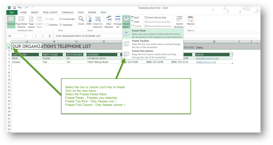 Under the View tab in the Window Group, click on the Freeze Panes command. This allows you to freeze the top row, far left column, or whatever you select. If you have to review a large database (for instance a privilege log), Freeze Panes can make for easier scrolling.
If you need to freeze the first row AND the first column select the header row and while holding down the Control key <Ctrl> select the first column. Then click “Freeze Panes”.
Add the Freeze Panes to your Quick Access toolbar so it is easy to find every time you need it!
Wrap Text
Text in a cell may become hidden by the column to the right if the contents are too long. To see all the text in a cell, select it and then press the Wrap Text button, in the Alignment group on the Home tab. You can also apply Wrap Text to an entire column or row by selecting it by its header. Wrap Text is great if you do not want to adjust the width of the columns.
Once you have applied Wrap Text to the column you can then apply Autofit to view all your data concisely. On the Home tab, under the Cells group, press the Format menu. Select Autofit Column Width and the columns will snap to the size of the contents they contain or select Autofit Row Height to tighten up the size of your rows.
Flash Fill
Whether you are sending data to an ediscovery vendor or repurposing data through a mail merge to a letter in MS Word, you can easily separate data with no formula required! Here’s a quick example of the power of Flash Fill courtesy Ben Schorr’s Facebook Group: Office for Lawyers
“One such problem is extracting a person’s first name from a column of full names. In a blank column adjacent to the one that contains full names, you simply type the first name and then click the Home tab, and select Fill, Flash Fill. The first names of everyone in the list will be entered into that that column immediately. You can use the same process to extract last names, to join first and last names, to extract months, days or years from dates and even extract values from cells. While you could have always done this with formulas, now Flash Fill ensures anyone can do it very quickly and easily.”
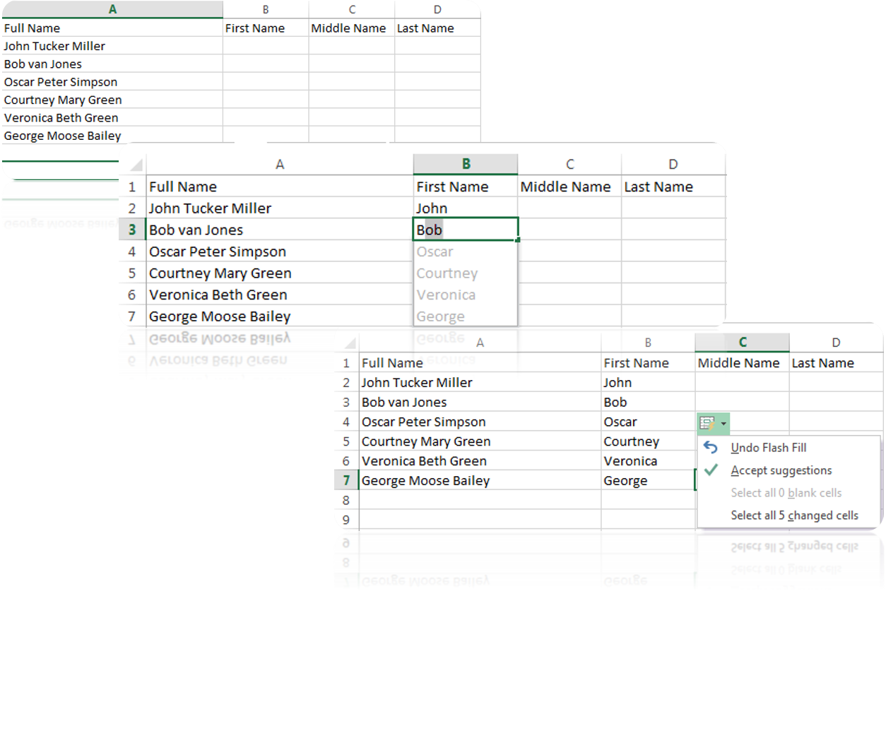 For instance, in the example above, you want to fill in the First Name, Middle Name and Last Name columns without having to type in all the data again. To do the First Name column, we will go to cell B2 and type John and then click <Enter>.
When you click <Enter> after entering John, Excel will move you to cell B3. Just type the first letter B and it will activate the Flash Fill feature.
Click <Enter> and the entire Column will be filled. A small icon will appear which you can use to access the Flash Fill options in case you wish to undo the action.
Need to do this in reverse and combine text from multiple columns into a single column? Try the TEXTJOIN formula!
Recommended Charts
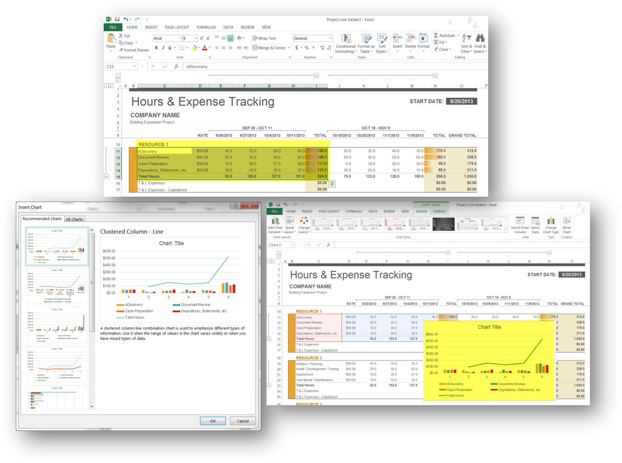
Why create a chart from scratch when you can ask Excel to build one for you? Follow the steps below to generate fast, beautiful charts that clearly showcase the data you’ve compiled.
- Select the data you’d like to create a chart for
- Click on Recommended Charts inside the Insert Menu
- Select the chart you would like to see
- Click OK
- Use the Chart Elements and filters to further change the data
 Similarly, a PivotTable allows you to ask a question of your data. It gets its name because you can “pivot” the data to display vertically or horizontally. It’s easy to create a PivotTable by going to the Insert Tab, selecting all your data, and then pressing “Pivot Table.” A menu will appear asking you if you want to place this PivotTable in a new worksheet or on the existing one.
Turn Text to Tables
To make quick work of sorting and filtering data in a spreadsheet convert the text to a table. First select your data, then on the Home tab, under the Styles group, select Format as Table and choose what looks best to you.
Excel will now give you some features that make manipulating this data much easier:
- Column headings are always visible.
- You can use AutoFilter to filter or sort columns of your list. It will sort everything all together at once, so you don’t run into the common problem where you sort one column, and then everything is no longer corresponding to the cells around it.
- Ledger Lines: Table Styles that make your data easier to see
- Hitting the Tab key in the last row of your table will now insert new blank rows into your table
- Table Tools Ribbon: shows more formatting and options to get the most out of the table
- View Total Row in Table Tools ribbon
Conclusion
From crunching numbers to sorting piles of data to presenting information, Excel can be handy for all types of reasons in a law office. Knowing a few tips to make formatting easier will help you master this powerful spreadsheet software. Want to learn more? GCFLearnFree has fantastic Excel tutorials and Microsoft also has a great Excel help database.